Causal Inference
Fill In Your Name
01 March 2022
- Why should social scientists and policymakers care about causality?
- Counterfactual Approach to Causal Inference
- Potential Outcomes
- Randomization of
treatment assignment
- Randomization of treatment assignment
- Random assignment vs. random sampling
- Randomization is powerful (1)
- Randomization is powerful (2)
- Randomization is powerful (3)
- Random sampling
- Potential outcomes
- Random assignment to red (1) or blue (0) condition
- Three key assumptions
- Key assumption: SUTVA, part 1
- Key assumption: SUTVA, part 2
- Key assumption: Excludability
- Randomization is powerful (4)
- Randomized vs. observational studies
Why should social scientists and policymakers care about causality?
- [Discussion with your own examples.]
Counterfactual Approach to Causal Inference
Recent changes in social science research
Historically, reverse causality and omitted variable bias have been problematic for a lot of social science research aimed at making causal claims.
Recently, the counterfactual approach has been embraced in the social sciences as a framework for causal inference.
This represents a big shift in research:
Being more precise about what we mean by causal effects.
Using randomization or designs with as-if randomization.
More partnerships between researchers and practitioners.
“X causes Y” is a claim about what didn’t happen
In the counterfactual approach: “If X had not occurred, then Y would not have occurred.”
Experiments help us learn about counterfactual and manipulation-based claims about causation.
It’s not wrong to conceptualize “cause” in another way. But it has been productive to work in this counterfactual framework (Brady 2008).
How to interpret “X causes Y” in this approach
“X causes Y” need not imply that W and V do not cause Y: X is a part of the story, not the whole story. (The whole story is not necessary in order to learn about whether X causes Y).
“X causes Y” requires a context: matches cause flame but require oxygen; small classrooms improve test scores but require experienced teachers and funding (Cartwright and Hardie 2012).
“X causes Y” can mean “With X, the probability of Y is higher than would be without X.” or “Without X there is no Y.” Either is compatible with the counterfactual idea.
How to interpret “X causes Y” in this approach
It is not necessary to know the mechanism to establish that X causes Y. The mechanism can be complex, and it can involve probability: X causes Y sometimes because of A and sometimes because of B.
Counterfactual causation does not require “a spatiotemporally continuous sequence of causal intermediates”
- Ex: Person A plans event Y. Person B’s action would stop Y (say, a random bump from a stranger). Person C doesn’t know about Person A or action Y but stops B (maybe thinks B is going to trip). So, Person A does action Y. And Person C causes action Y (without Person C’s action, Y would not have occurred) (Holland 1986).
Correlation is not causation.
Exercise: Echinacea
Your friend says taking echinacea (a traditional remedy) reduces the duration of colds.
If we take a counterfactual approach, what does this statement implicitly claim about the counterfactual? What other counterfactuals might be possible and why?
Potential Outcomes
Potential outcomes
For each unit we assume that there are two post-treatment outcomes: \(Y_i(1)\) and \(Y_i(0)\).
\(Y_i(1)\) is the outcome that would obtain if the unit received the treatment (\(T_i=1\)).
\(Y_i(0)\) is the outcome that would obtain if the unit received the control (\(T_i=0\)).
Definition of causal effect
The causal effect of treatment (relative to control) is: \(\tau_i = Y_i(1) - Y_i(0)\)
Note that we’ve moved to using \(T\) to indicate our treatment (what we want to learn the effect of). \(X\) will be used for background variables.
Key features of this definition of causal effect
You have to define the control condition to define a causal effect.
- Say \(T=1\) means a community meeting to discuss public health. Is \(T=0\) no meeting at all? Is \(T=0\) a community meeting on a different subject? Is \(T=0\) a flyer on public health?
- The phrase ``causal effect of \(T\) on \(Y\)’’ doesn’t make sense without knowing what is means to not have \(T\).
Each individual unit \(i\) has its own causal effect \(\tau_i\).
But we can’t measure the individual-level causal effect, because we can’t observe both \(Y_i(1)\) and \(Y_i(0)\) at the same time. This is known as the fundamental problem of causal inference. What we observe is \(Y_i\):
\(Y_i = T_iY_i(1) + (1-T_i)Y_i(0)\)
Imagine we know both \(Y_i(1)\) and \(Y_i(0)\) (this is never true!)
| \(i\) | \(Y_i(1)\) | \(Y_i(0)\) | \(\tau_i\) |
|---|---|---|---|
| Andrei | 1 | 1 | 0 |
| Bamidele | 1 | 0 | 1 |
| Claire | 0 | 0 | 0 |
| Deepal | 0 | 1 | -1 |
We have the treatment effect for each individual.
Note the heterogeneity in the individual-level treatment effects.
But we only have at most one potential outcome for each individual, which means we don’t know these treatment effects.
Average causal effect
- While we can’t measure the individual causal effect, \(\tau_i = Y_i(1)-Y_i(0)\), we can randomly assign subjects to treatment and control conditions to estimate the average causal effect, \(\bar{\tau}_i\):
\(\overline{\tau_i} = \frac{1}{N} \sum_{i=1}^N ( Y_i(1)-Y_i(0) ) = \overline{Y_i(1)-Y_i(0)}\)
The average causal effect is also known as the average treatment effect (ATE).
Further explanation on how after we discuss randomization of treatment assignment in the next section.
Estimands and causal questions
Before we discuss randomization and how that allows us to estimate the ATE, note that the ATE is a type of estimand.
An estimand is a quantity you want to learn about (from your data). It’s the target of your research that you set.
Being precise about your research question means being precise about your estimand. For causal questions, this means specifying:
- The outcome
- The treatment and control conditions
- The study population
Other types of estimands you may be interested in
The ATE for a particular subgroup, aka conditional average treatment effect (CATE)
Differences in CATEs: differences in the average treatment effect for one group as compared with another group.
The ATE for just the treated units, aka ATT (average treatment effect on the treated)
The local ATE (LATE). “Local” = those whose treatment status would be changed by an encouragement in an encouragement design (aka CACE, complier average causal effect) or those in the neighborhood of a discontinuity for a regression discontinuity design.
Estimands are discussed in detail in Estimands and Estimators Module.
Randomization of treatment assignment
Randomization of treatment assignment
Randomization means that every observation has a known probability of assignment to experimental conditions between 0 and 1.
- No unit in the experimental sample is assigned to treatment with certainty (probability = 1) or to control with certainty (probability = 0).
Units can vary in their probability of treatment assignment.
For example, the probability might vary by group: women might have a 25% probability of being assigned to treatment while men have a different probability.
It can even vary across individuals, though that would complicate your analysis.
Random assignment vs. random sampling
Randomization (of treatment): assigning subjects with known probability to experimental conditions.
This random assignment of treatment can be combined with any kind of sample (random sample, convenience sample, etc.).
But the size and other characteristics of your sample will affect your power and your ability to extrapolate from your finding to other populations.
Random sampling (from population): selecting subjects into your sample from a population with known probability.
Randomization is powerful (1)
We want the ATE, \(\overline{\tau_i}= \overline{Y_i(1)-Y_i(0)}\).
We will make use of the fact that the average of differences equals the difference of averages:
ATE \(= \overline{Y_i(1)-Y_i(0)} = \overline{Y_i(1)}-\overline{Y_i(0)}\)
Randomization is powerful (2)
Let’s randomly assign some of our units to the treatment condition. For these treated units, we measure the outcome \(Y_i|T_i=1\), which is the same as \(Y_i(1)\) for these units.
Because these units were randomly assigned to treatment, these \(Y_i=Y_i(1)\) for the treated units represent the \(Y_i(1)\) for all our units.
In expectation (or on average across repeated experiments (written \(E_R[]\))):
\(E_R[\overline{Y_i}|T_i=1]=\overline{Y_i(1)}\).
\(\overline{Y}|T_i=1\) is an unbiased estimator of the population mean of potential outcomes under treatment.
The same logic applies for units randomly assigned to control:
\(E_R[\overline{Y_i}|T_i=0]=\overline{Y_i(0)}\).
Randomization is powerful (3)
- So we can write down an estimator for the ATE:
\(\hat{\overline{\tau_i}} = ( \overline{Y_i(1)} | T_i = 1 ) - ( \overline{Y_i(0)} | T_i = 0 )\)
- In expectation, or on average across repeated experiments, \(\hat{\overline{\tau_i}}\) equals the ATE:
\(E_R[Y_i| T_i = 1 ] - E_R[Y_i | T_i = 0] = \overline{Y_i(1)} - \overline{Y_i(0)}\).
- So we can just take the difference of these unbiased estimators of \(\overline{Y_i(1)}\) and \(\overline{Y_i(0)}\) to get an unbiased estimate of the ATE.
Random sampling
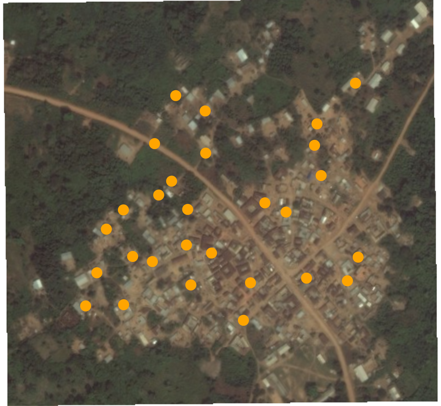
Random sample of households
Potential outcomes
Each household \(i\) has \(Y_i(1)\) and \(Y_i(0)\).
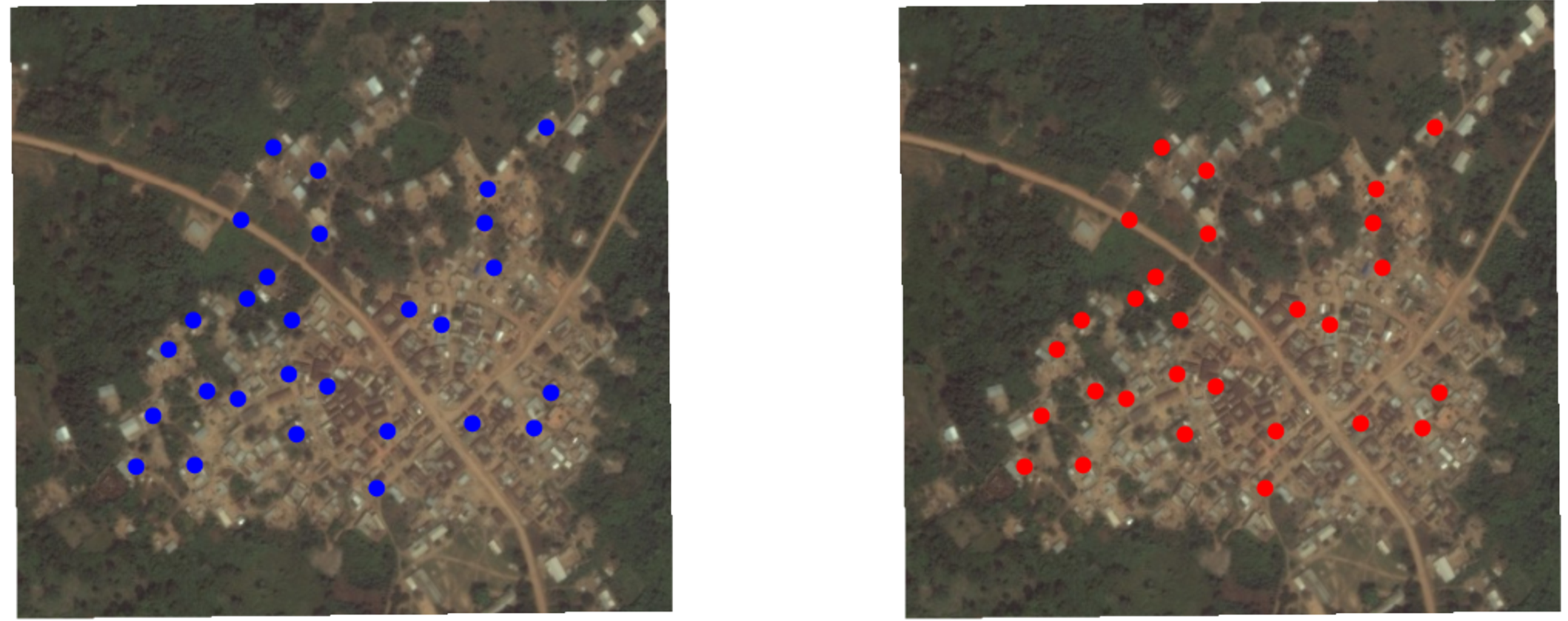
Random assignment to red (1) or blue (0) condition
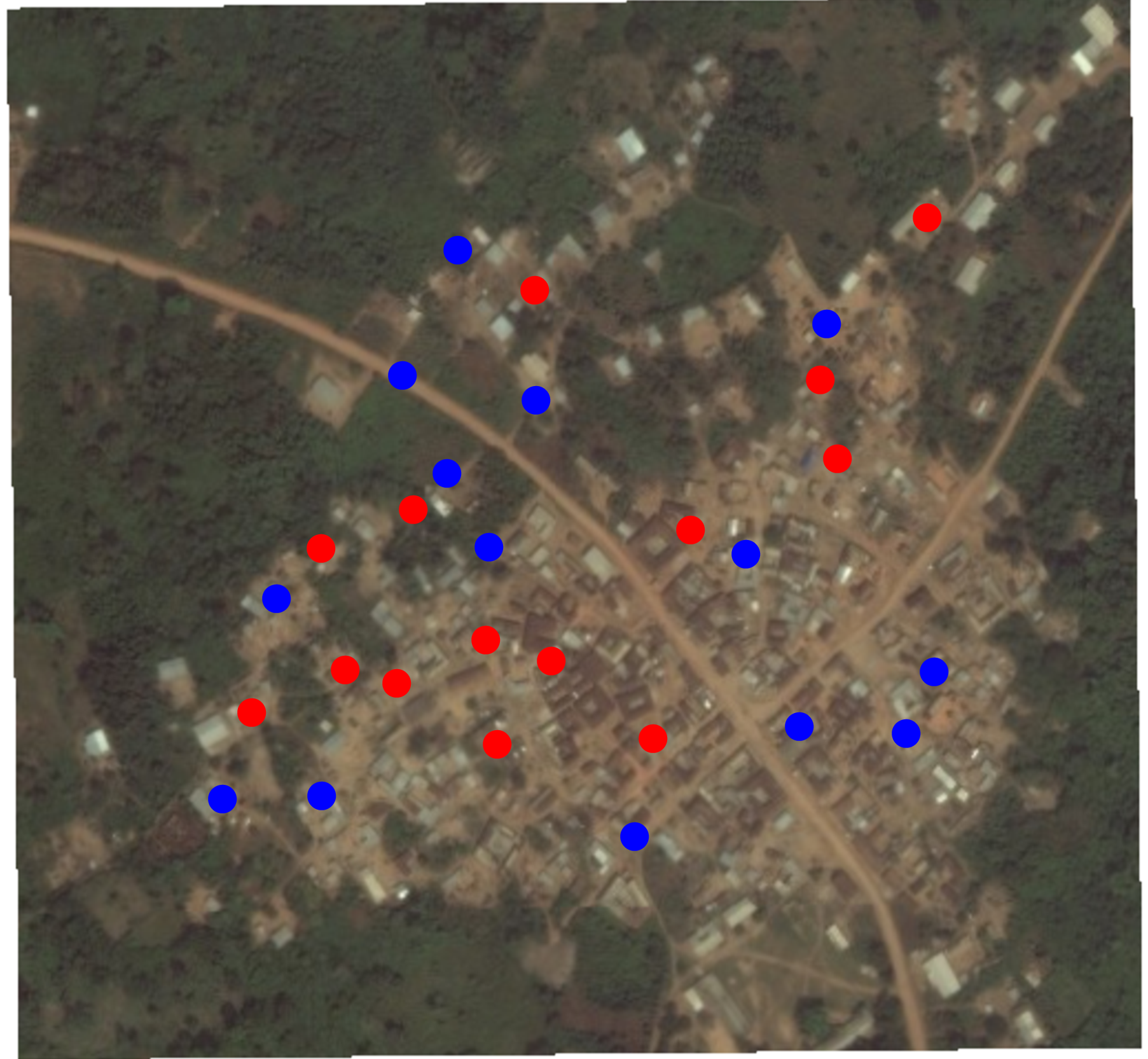
Random assignment of this random sample of households
Three key assumptions
To make causal claims with an experiment (or to judge whether we believe a study’s claims), we need three core assumptions:
Random assignment of subjects to treatment, which implies that receiving the treatment is statistically independent of subjects’ potential outcomes.
Stable unit treatment value assumption (SUTVA).
Excludability, which means that a subject’s potential outcomes respond only to the defined treatment, not other extraneous factors that may be correlated with treatment.
Key assumption: SUTVA, part 1
No interference – A subject’s potential outcome reflects only whether that subject receives the treatment himself/herself. It is not affected by how treatments happen to be allocated to other subjects.
A classic violation is the case of vaccines and their spillover effects.
Say I am in the control condition (no vaccine). If whether I get sick (\(Y_i(0)\)) depends on other people’s treatment status (whether they take the vaccine), it’s like I have two different \(Y_i(0)\)!
SUTVA (= stable unit treatment value assumption)
Key assumption: SUTVA, part 2
No hidden variations of the treatment
Say treatment is taking a vaccine, but there are two kinds of vaccines and they have different ingredients.
An example of a violation is when whether I get sick when I take the vaccine (\(Y_i(1)\)) depends on which vaccine I got. We would have two different \(Y_i(1)\)!
Key assumption: Excludability
Treatment assignment has no effect on outcomes except through its effect on whether treatment was received.
Important to define the treatment precisely.
Important to also maintain symmetry between treatment and control groups (e.g., through blinding, having the same data collection procedures for all study subjects, etc.), so that treatment assignment only affects the treatment received, not other things like interactions with researchers that you don’t want to define as part of the treatment.
Randomization is powerful (4)
If the intervention is randomized, then who receives or doesn’t receive the intervention is not related to the characteristics of the potential recipients.
Randomization makes those who were randomly selected to not receive the intervention to be good stand-ins for the counterfactuals for those who were randomly selected to receive the treatment, and vice versa.
We have to worry about this if the intervention were not randomized (= an observational study).
Randomized vs. observational studies
Different types of studies
Randomized studies
- Randomize treatment, then go measure outcomes
Observational studies
- Treatment is not randomly assigned. It is observed, but not manipulated.
Exercise: Learning about your prior knowledge
Discuss in small groups: Help me design the next project to answer one of these questions (or one of your own causal questions). Just sketch the key features of two designs — one observational and the other randomized.
Example research questions:
Do Community-Driven Reconstruction projects increase trust and cooperation in Liberia? see EGAP Policy Brief 40
Can community monitoring increase clinic utilization and decrease child mortality in Uganda? see EGAP Policy Brief 58
Exercise: Observational studies vs. Randomized studies
Tasks:
Sketch an ideal observational study design (no randomization, no researcher control but infinite resources for data collection). What questions would critical readers ask when you claim that your results reflect a causal relationship?
Sketch an ideal experimental study design (including randomization). What questions would critical readers ask when you claim that your results reflect a causal relationship?
Discuss
What were key components and strengths and weaknesses of the randomized studies?
What were key components and strengths and weaknesses of the observational studies?
Generalizability and external validity
Randomization brings high internal validity to a study – confidence that we have learned the causal effect of a treatment on an outcome.
But the finding from a particular study in one particular place and at one particular time may not hold in other settings (i.e., external validity).
This is a general concern, not just a concern for randomized studies.
EGAP’s Metaketa Initiative works to accumulate knowledge by pre-planning a meta-analysis of multiple studies that have high internal validity due to randomization.
References
EGAP Policy Brief 40: Development Assistance and Collective Action Capacity
EGAP Policy Brief 58: Does Bottom-Up Accountability Work?