Hypothesis Testing: Summarizing Information about Causal Effects
Fill In Your Name
01 March 2022
- The Role of Hypothesis Tests in Causal Inference
- Hypothesis Testing Basics
- Ingredients of a hypothesis test
- A hypothesis is a statement about or model of a relationship between potential outcomes
- Test statistics summarize treatment-to-outcome relationships
- The design links test statistic and hypothesis
- The design guides creation of a distribution of hypothetical test statistics
- Plot the randomization distributions under the null
- \(p\)-values summarize the plots
- How to do this in R: COIN
- How to do this in R: RItools
- How to do this in R: RI2
- Next topics
- Testing weak null hypotheses
- Rejecting null hypotheses
- Rejecting hypotheses and making errors
- False positive rates in hypothesis testing
- False positive and false negative errors
- A single test of a single hypothesis
- Decisions imply errors
- Diagnosing false positive rates by simulation
- Diagnosing false positive rates by simulation
- Diagnosing false positive rates by simulation
- Diagnosing false positive rates by simulation
- Diagnosing false positive rates by simulation
- False positive rate with \(N=60\) and binary outcome
- False positive rate with \(N=60\) and continuous outcome
- Summary
- Advanced Topics
- Testing many hypotheses
- When might we test many hypotheses?
- False positive rates in multiple hypothesis testing
- Discoveries with multiple tests
- Two main error rates to control when testing many hypotheses
- Questions with multiple outcomes
- Multiple hypothesis testing: Multiple Outcomes
- Can we detect an
effect on outcome
Y1? - On which of the five outcomes can we detect an effect?
- Can we detect an effect for any of the five outcomes?
- Comparing approaches I
- Comparing approaches II
- The Holm correction
- Multiple hypothesis testing: Multiple treatment arms
- Multiple hypothesis testing: Multiple treatment arms
- Multiple hypothesis testing: Multiple treatment arms
- Approaches to testing hypotheses with multiple arms
- Summary
- References
Plot the randomization distributions under the null
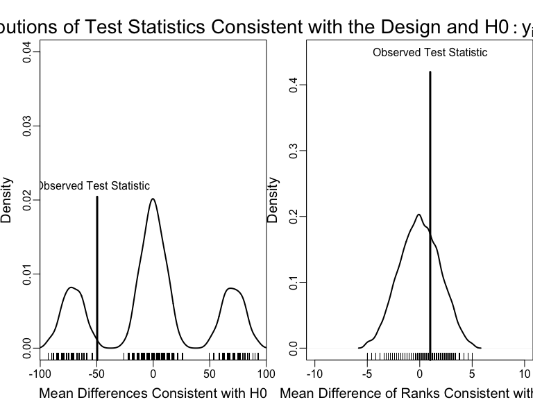
An example of using the design of the experiment to test a hypothesis with two different test statistics.
Testing the weak null of no average effects
Both variation and location of \(Y\) changes with treatment in this simulation.
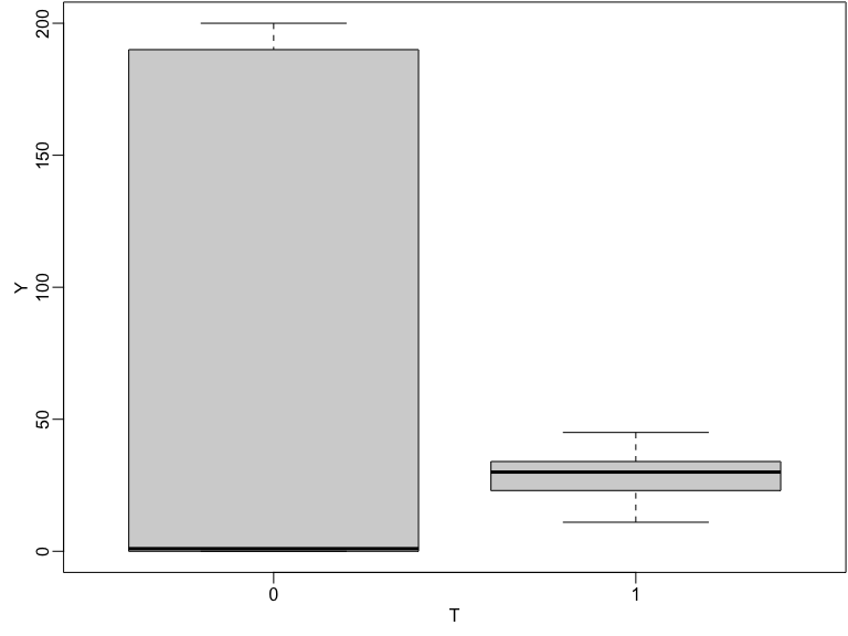
Boxplot of observed outcomes by treatment status
False positive rates in hypothesis testing
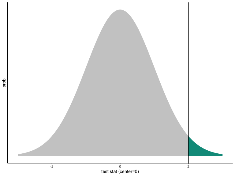
One-sided p-value from a Normally distributed test statistic.
Notice:
The curve is centered at the hypothesized value.
The curve represents the world of the hypothesis.
The \(p\)-value is how rare it would be to see the observed test statistic (or a value farther away from the hypothesized value) in the world of the null.
In the picture, the observed value of the test statistic is consistent with the hypothesized distribution, but just not super consistent.
Even if \(p < .05\) (or \(p < .001\)) the observed test statistic must reflect some value on the hypothesized distribution. This means that you can always make an error when you reject a null hypothesis.
Diagnosing false positive rates by simulation
Compare tests by plotting the proportion of p-values less than any given number. The “randomization inference” tests control the false positive rate (these are the tests of using direct permutation, repeating the experiment).
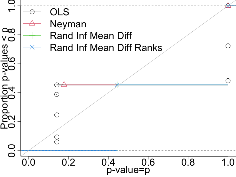
P-value distributions when there are no effects for four tests with n=10. A test that controls its false positive rate should have points on or below the diagonal line.
False positive rate with \(N=60\) and binary outcome
In this design only the direct randomization inference-based tests control the false positive rate.
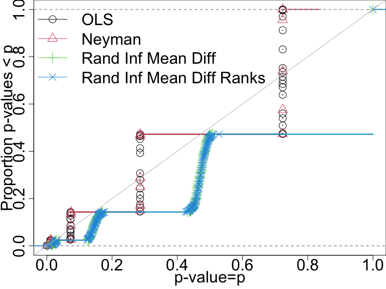
P-value distributions when there are no effects for four tests with n=60 and a binary outcome. A test that controls its false positive rate should have points on or below the diagonal line.
False positive rate with \(N=60\) and continuous outcome
Here, all of the tests do a good job of controlling the false positive rate.
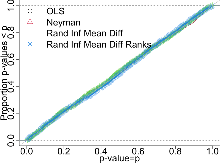
P-value distributions when there are no effects for four tests with n=60 and a continuous outcome. A test that controls its false positive rate should have points on or below the diagonal line.