B Introduction to R and RStudio
Throughout the book we include R code for estimation, simulation, and creating examples. We used RStudio to create the slides. To personalize them for your own purpose, we assume you will use R Markdown. Below, we include guides to setting up R and RStudio on your machine, as well as some basic commands that are frequently used.
B.1 R and RStudio
R is a free software environment most commonly used for statistical analysis and computation. Because Learning Days participants arrive with different statistical backgrounds and preferred statistical software, we use R to ensure that everyone is on the same page. We advocate the use of R more generally for its flexibility, wealth of applications, and comprehensive support mostly through online fora.
RStudio is a free, open source integrated development environment with a user interface that makes R much more user-friendly. R Markdown, a feature of RStudio, enables the easy output of code, results, and text in a .pdf, .html, or .doc format.
B.2 Downloading R and RStudio
B.2.1 Downloading R
R can be freely downloaded from CRAN at the link corresponding to your operating system:
- For Windows: https://cran.r-project.org/bin/windows/base/
- For Mac OS X: https://cran.r-project.org/bin/macosx/.
- Select
R-4.2.1.pkgfor OS X 10.13 and higher. - Select
R-3.6.3.nnpkgfor OS X 10.11-10.12. - Select
R-3.3.3.nnpkgfor OS X 10.19-10.10. - Select
R-3.2.1-snowleopard.pkgfor OS X 10.6-10.8.
- Select
B.2.2 Downloading RStudio
RStudio can be freely downloaded from the RStudio website, https://www.rstudio.com/products/rstudio/download/. In the table, click the blue Download button at the top of the left column, “RStudio Desktop Open Source License” as depicted below in Figure B.1. Once you select this button, the page will jump to a list of download options as depicted in Figure B.2.
- For Windows, select
Windows 10/8/7. - For Mac OS X, select
Mac OS X 10.13+.
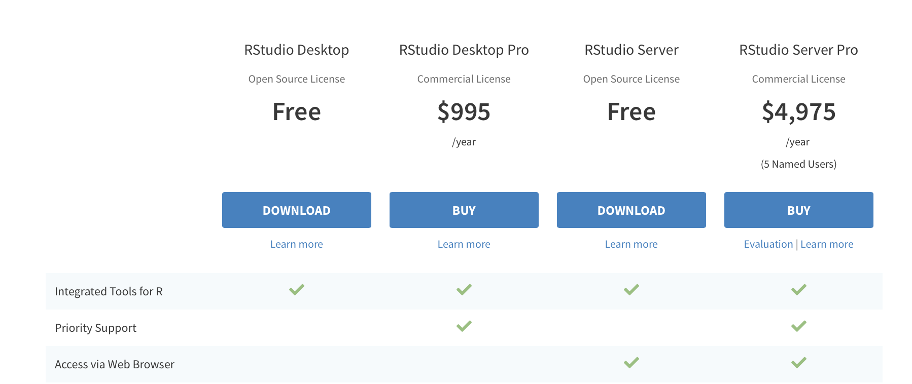
Figure B.1: Select Download in the “RStudio Desktop Open Source License” column.
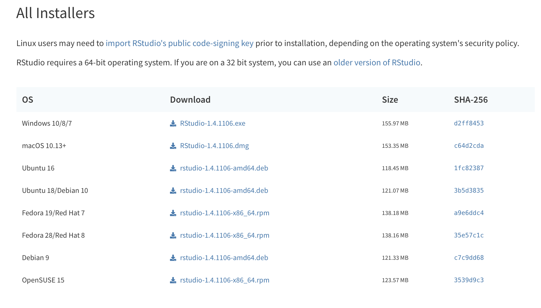
Figure B.2: Select the Windows 10/8/7 link for Windows or the Mac OS X 10.13+ link for Mac.
B.3 RStudio Interface
When you open RStudio for the first time, there should be three panels visible, as depicted in Figure B.3 below.
- Console (left panel)
- Accounting (upper right panel): includes Environment and History tabs
- Miscellaneous (lower right panel)
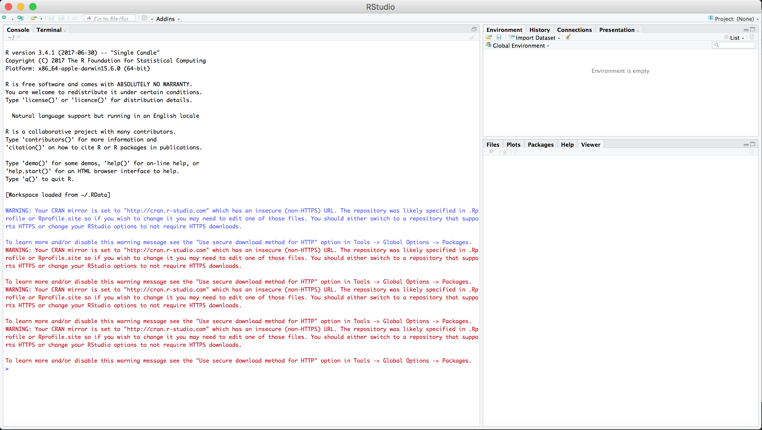
Figure B.3: When you open RStudio, there are three panels visible: the Console (left), Accounting (upper right), and Miscellaneous (lower right).
B.3.1 Console
You can execute all operations in the console. For example if you enter 4 + 4 and hit the Enter/Return key, the Console will return [1] 8.
To make sure everyone is prepared to use R at Learning Days, we ask participants to run one line of code in the Console to download several R packages. Packages are fragments of reproducible code that allow for more efficient analysis in R. To run these lines, copy the following code into the Console and hit your Return/Enter key. You must be connected to the internet to download packages.
install.packages(c("ggplot2", "dplyr", "AER", "arm", "MASS", "sandwich",
                   "lmtest", "estimatr","coin","randomizr", "DeclareDesign"))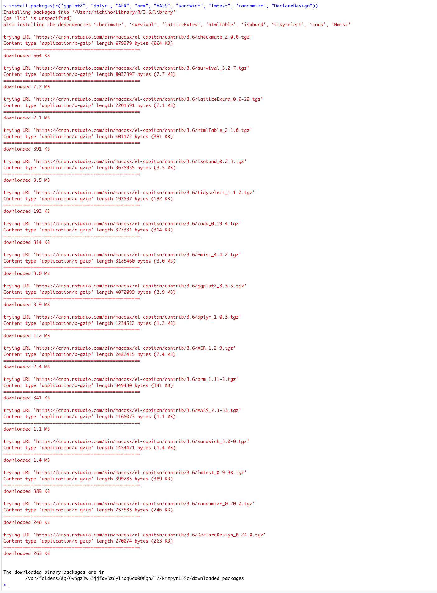
Figure B.4: An image of the Console after executing the three lines of code listed above.
B.3.2 Editor
In order to write and save reproducible code, we will open a fourth panel, the Editor, by clicking on the icon with a white page with a plus sign on the upper-left corner of the RStudio interface and selecting R Script, as depicted in Figure B.5.
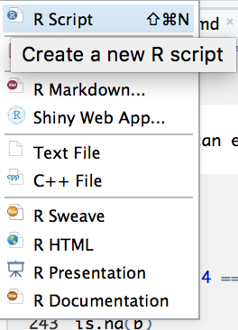
Figure B.5: Create a new R script and open the editor panel by selecting R Script from the dropdown menu.
Once the R script is opened, there should be four panels within the RStudio interface, now with the addition of the Editor panel. We can execute simple arithmetic by entering a formula in the editor and pressing Control + Enter (Windows) or Command + Enter (Mac). The formula and the “answer” will appear in the Console, as depicted in Figure B.6, with red boxes added for emphasis.
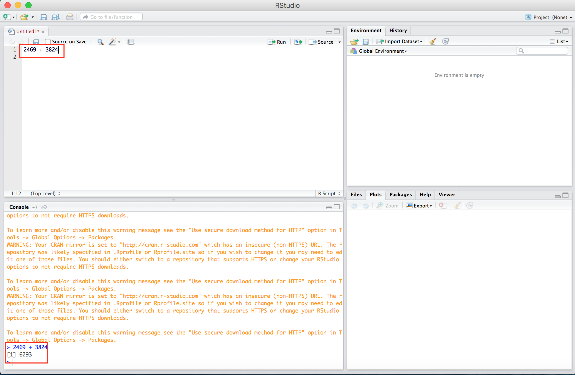
Figure B.6: An arithmetic expression is entered in the editor and evaluated in the console. The red boxes are added for emphasis.
R can be used for any arithmetic operation including, but not limited to, addition (+), subtraction (-), scalar multiplication (*), division (/), and exponentiation (^).
B.3.3 Accounting
Beyond basic functions, we can also store values, data, and functions in the global environment. To assign a value to a variable, use the <- operator. All stored values, functions, and data will appear in the Environment tab in the Accounting panel. In Figure B.7, we define the variable t to take the value \(3 \times \frac{6}{14}\), and can see that it is stored under Values.
We also load a dataset. Here, “ChickWeight” is a dataset built into R; most datasets will be loaded from the web or other files on your computer through an alternate method. We can see that ChickWeight contains 578 observations of 4 variables and is stored in the Environment. By clicking on the name ChickWeight a tab will enter with the dataset in your Editor window.
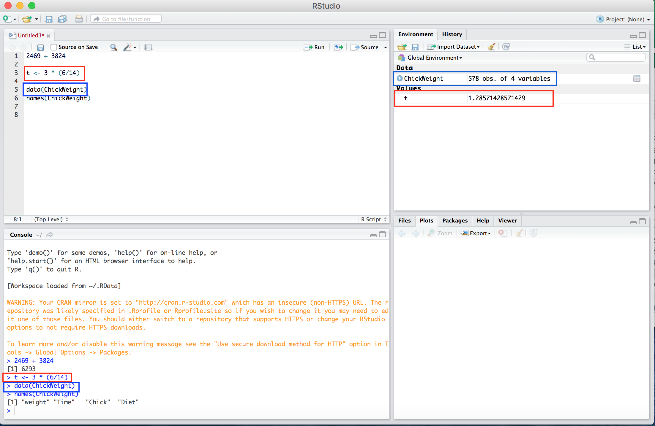
Figure B.7: The value 3 * (6/14) is assigned to the variable t (red) and the dataset ChickWeight is added to the global environment (blue). The boxes are added for emphasis.
The Learning Days workshops use many tools in R to analyze and view data. For now, we can learn some basic tools to examine the data. The function head() allows us to see the first six rows of the dataset. summary() summarizes each of the columns of the dataset and dim() provides the dimensions of the dataset with first the number of rows and then columns.
head(ChickWeight) # First 6 observations in dataset weight Time Chick Diet
1 42 0 1 1
2 51 2 1 1
3 59 4 1 1
4 64 6 1 1
5 76 8 1 1
6 93 10 1 1summary(ChickWeight) # Summary of all variables weight Time Chick Diet
Min. : 35 Min. : 0.0 13 : 12 1:220
1st Qu.: 63 1st Qu.: 4.0 9 : 12 2:120
Median :103 Median :10.0 20 : 12 3:120
Mean :122 Mean :10.7 10 : 12 4:118
3rd Qu.:164 3rd Qu.:16.0 17 : 12
Max. :373 Max. :21.0 19 : 12
(Other):506 dim(ChickWeight) # Dimensions of the dataset in the order rows, columns[1] 578 4Unlike other statistical software, R allows users to store multiple datasets, possibly of different dimensions, simultaneously. This feature makes R quite flexible for analysis using multiple methods.
B.3.4 Miscellaneous
R provides a suite of tools, ranging from built-in plot functions to packages to graph data, models, estimates, etc. The final Miscellaneous panel allows for the quick viewing of graphs in RStudio. Figure B.8 shows a plot in this panel. Leaning Days will discuss how to plot data; for now, don’t worry about the graphing the code in the Editor.
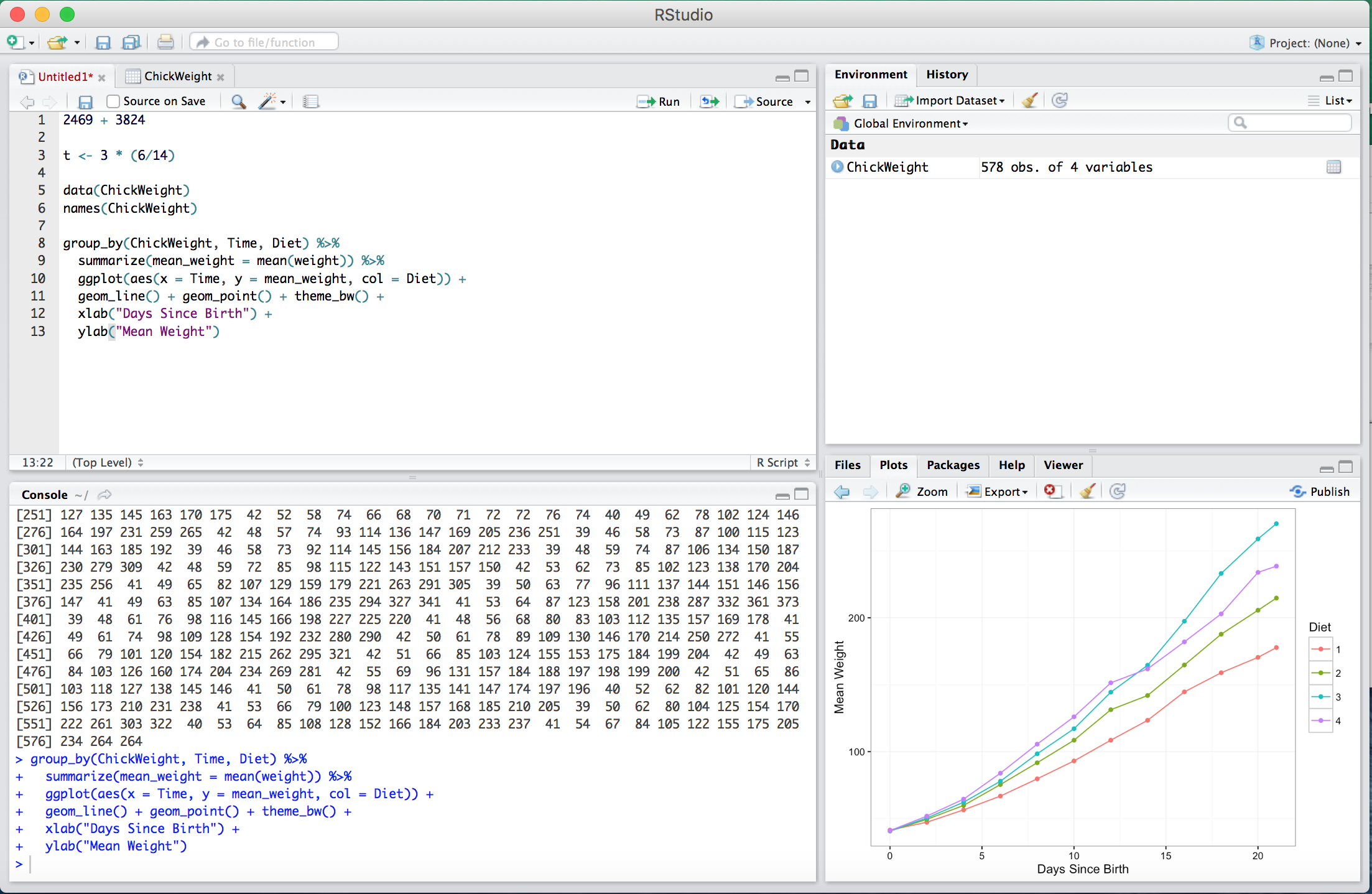
Figure B.8: An example plot of the ChickWeight data made in R.
B.4 Learning to Use R
B.4.1 Online Resources
There are many helpful online resources to help you start learning R. We recommend two sources:
- Code School, which runs entirely through your browser https://www.codeschool.com/courses/try-r.
- Coursera, via an online R Programming course organized by Johns Hopkins University:
- Go to https://www.coursera.org
- Create an account (this is free!)
- Sign up for R Programming at Johns Hopkins University (instructor: Roger Peng) under the “Courses” tab
- Read the materials and watch the videos from the first week. The videos from the first week are about 2.5 hours long total.
B.4.2 Basic Practice
Here we provide some fragments of code to familiarize you with some basic practices in R. We recommend that you practice by typing the code fragments into your Editor and then evaluating them.
B.4.2.1 Setting up an R Session
In general, we read other files such as data or functions into R and output results like graphs or tables into files not contained within an R session. To do this, we must give R an “address” at which it can locate such files. It may be most efficient to do this by setting a working directory, a file path at which relevant files are stored. We can identify the current working directory using getwd() and set a new one using setwd(). Note that the syntax of these filepaths varies by operating system.
getwd()setwd("~TaraLyn/EGAP Learning Days Admin/Workshop 2018_2 (Uruguay)/") You may need to install packages beyond those listed above to execute certain functions. To install packages we use install.packages(""), filling in the package name between the "" marks, as follows. You need only install packages once.
install.packages("randomizr") Once a package is installed, it can be loaded and accessed using library() where the package name is inserted between the parentheses (no "" marks).
library(randomizr)To clear R’s memory of the stored data, functions, or values that appear in the accounting tab, use rm(list = ls()). It may be useful to set a random number seed to ensure that replication is possible in a different R session, particularly when we work with simulation-based methods.
rm(list = ls())
set.seed(2018)  # Optional: Set a seed to make output replicable
B.4.2.2 R Basics
We now explore some basic commands. In order to assign a scalar (single element) to a variable, we use the <- command as discussed previously:
# "<-"  is the assignment command; it is used to define things. eg:
(a <- 5)
[1] 5We may also want to assign a vector of elements to a variable. Here we use the same <- command, but focus on how to create the vector.
(b <- 1:10) # ":" is used to define a string of integers [1] 1 2 3 4 5 6 7 8 9 10(v <- c(1, 3, 2, 4, pi)) # use c() to make a vector with anything in it[1] 1.000 3.000 2.000 4.000 3.142We can then refer to elements of a vector by denoting their position in a vector inside hard brackets [].
# Extract elements of a vector:
b[1]                   # Returns position 1
[1] 1b[5:4] # Returns positions 5 and 4, in that order[1] 5 4b[-1] # Returns all but the first number [1] 2 3 4 5 6 7 8 9 10# Returns all numbers indicated as "TRUE"
b[c(TRUE, FALSE, TRUE, FALSE, FALSE, TRUE, TRUE, FALSE, FALSE, FALSE)] [1] 1 3 6 7# Assign new values to particular elements of a vector
b[5] <- 0There are a set of built-in functions that can be applied to vectors like b.
sum(b) # Sum of all elements[1] 50mean(b) # Mean of all elements[1] 5max(b) # Maximum of all elements[1] 10min(b) # Minimum of all elements[1] 0sd(b) # Standard deviation of all elements[1] 3.496var(b) # Variance of all elements[1] 12.22We can also apply arithmetic transformations to all elements of a vector:
b^2 # Square the variable [1] 1 4 9 16 0 36 49 64 81 100b^.5 # Square root of the variable [1] 1.000 1.414 1.732 2.000 0.000 2.449 2.646 2.828 3.000 3.162log(b) # Log of variable [1] 0.0000 0.6931 1.0986 1.3863 -Inf 1.7918 1.9459 2.0794 2.1972 2.3026exp(b) # e to the b [1] 2.718 7.389 20.086 54.598 1.000 403.429 1096.633 2980.958 8103.084 22026.466Finally, we can evaluate logical statements (i.e. ``is condition X true?’’) on all elements of a vector:
b == 2 # Is equal to [1] FALSE TRUE FALSE FALSE FALSE FALSE FALSE FALSE FALSE FALSEb < 5 # Less than [1] TRUE TRUE TRUE TRUE TRUE FALSE FALSE FALSE FALSE FALSEb >= 5 # Greater than or equal to [1] FALSE FALSE FALSE FALSE FALSE TRUE TRUE TRUE TRUE TRUEb <= 5 | b / 4 == 2 # | means OR [1] TRUE TRUE TRUE TRUE TRUE FALSE FALSE TRUE FALSE FALSEb>2 & b<9 # & means AND [1] FALSE FALSE TRUE TRUE FALSE TRUE TRUE TRUE FALSE FALSEis.na(b) # Indicates if data is missing [1] FALSE FALSE FALSE FALSE FALSE FALSE FALSE FALSE FALSE FALSEwhich(b<5) # Gives indices of values meeting logical requirement[1] 1 2 3 4 5The basic logic of these commands applies to data structures much more complex than scalars and vectors. Understanding of these basic features will help facilitate your understanding of more advanced topics during Learning Days.