For each unit, flip a coin to see if it will be treated. Then you measure outcomes at the same level as the coin.
The coins don’t have to be fair (50-50), but you have to know the probability of treatment assignment.
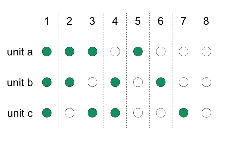
4.3 1. Simple randomization (coin-flipping)
4.4 1. Simple randomization (coin-flipping)
Advantage: Simple randomization can handle not knowing the total size of your sample in advance.
Disadvantage: You can’t guarantee a specific number of treated units and control units.
simple_ra(3)
[1] 0 1 1
simple_ra(3)
[1] 0 0 0
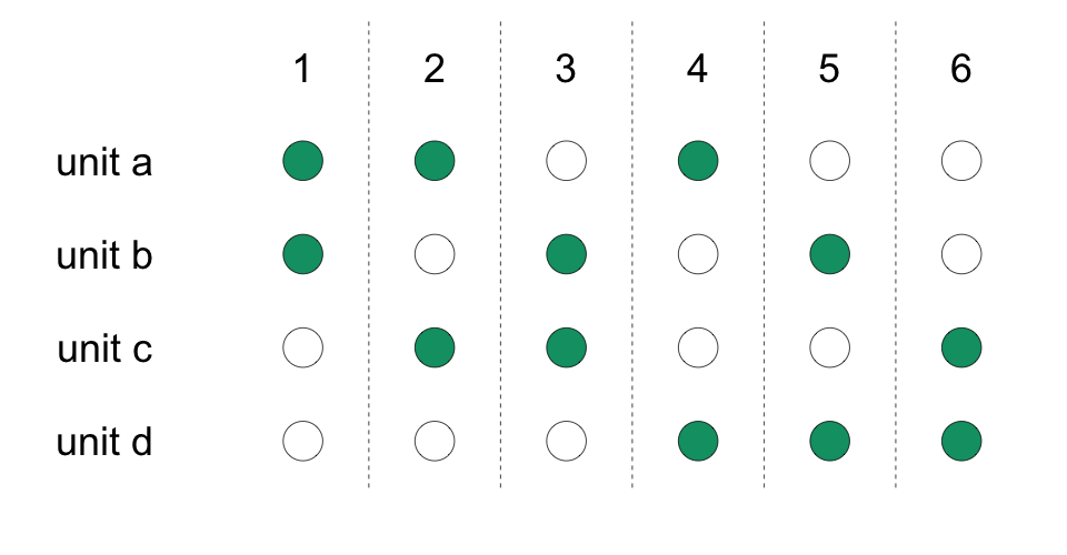
4.5 2. Complete randomization (drawing from an urn)
A fixed number \(m\) out of \(N\) units are assigned to treatment.
The probability a unit is assigned to treatment is \(m/N\).
This is like having an urn or bowl with \(N\) balls, of which \(m\) are marked as treatment and \(N-m\) are marked as control. Public lotteries use this method.
4.6 2. Complete randomization (drawing from an urn)
4.7 2. Complete randomization (drawing from an urn)
Advantage: Particularly useful when you have a small number of units to avoid having all units in only one condition.
Disadvantage: You need to know the total number of units in advance.
complete_ra(4)
[1] 0 0 1 1
complete_ra(4)
[1] 0 0 1 1
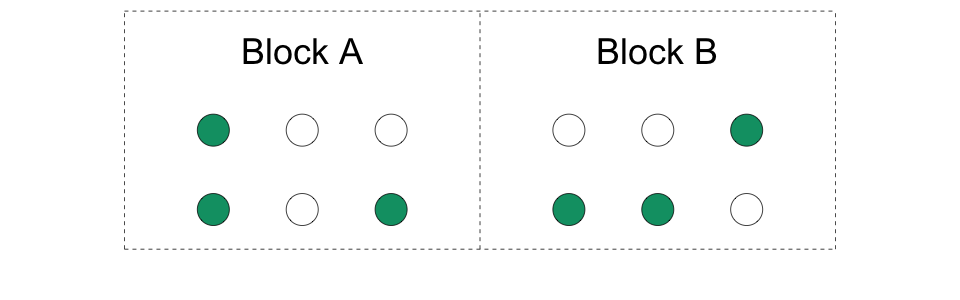
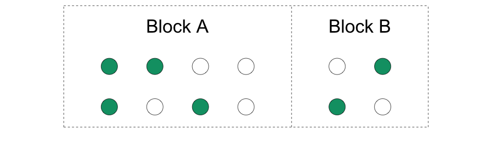
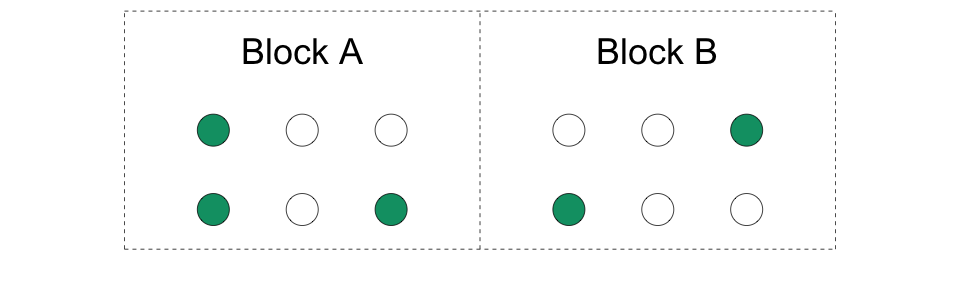
4.8 3. Block (or stratified) randomization
We create groups of units (blocks) and randomize separately within each block.
We are doing mini-experiments in each block so we have both treated and control units in each block.
4.9 3. Block (or stratified) randomization
Example: block = region, units = municipalities. We randomize treatment at the municipality level within region and also measure outcomes at the municipality level.
4.10 3. Block (or stratified) randomization
Blocks can be of different sizes.
4.11 3. Block (or stratified) randomization
Blocks can have different probabilities of treatment assignment.
4.12 3. Block (or stratified) randomization
How should you define your blocks?
Create subgroups for which you want to learn the ATE. The average causal effect for a particular subgroup is known as a Conditional Average Treatment Effect (CATE). You can use these to learn differences in CATEs for one group as compared with another group.
4.13 3. Block (or stratified) randomization
How should you define your blocks?
By variables that predict the outcome. This will increase the precision of your estimates.
4.14 3. Block (or stratified) randomization
Advantage: You avoid unlucky randomizations that create treatment and control groups that differ on the variables used to create the blocks. Blocks are generally very helpful.
This is especially useful for rare subgroups.
But we need data to form the blocks before the randomization.
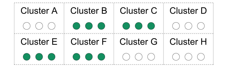
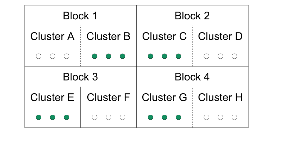
In a cluster-randomized study, all units in a group of units (the cluster) are assigned to the same treatment status.
4.17 4. Cluster randomization
Treatment is randomized at the cluster level.
Outcomes are measured at the unit level.
4.18 4. Cluster randomization
When should you do cluster randomization? If the intervention has to work at the cluster level.
Don’t if you can avoid it! Cluster randomization generally reduces statistical power. How much depends on the intra-cluster correlation (ICC or \(\rho\)). Higher \(\rho\) is worse.
4.19 4. Cluster randomization
If you must use cluster randomization, having more clusters helps.
Having fewer clusters hurts our ability to detect treatment effects and may cause misleading \(p\)-values and confidence intervals (or even estimates).